With the great success of deep learning, the demand for deploying deep neural networks to mobile devices is growing rapidly. Similar to what we do in desktop platforms, utilizing GPU in mobile devices can benefit both inference speed and energy efficiency. However, most existing deep learning frameworks do not support mobile GPU very well. The difficulty lies at the difference between mobile GPU architecture and desktop GPU architecture. It means special effort is required for optimizing on mobile GPU. The non-trivial extra work eventually results in the poor support of mobile GPU in most deep learning frameworks.
TVM addresses the difficulty of deploying for different hardwares by introducing an unified IR stack, with which the optimization for different hardwares can be done easily. In this post, we show how we use TVM/NNVM to generate efficient kernels for ARM Mali GPU and do end-to-end compilation. In our test on Mali-T860 MP4, compared with Arm Compute Library, our method is 1.4x faster on VGG-16 and 2.2x faster on MobileNet. Both graph-level and operator-level optimization contribute to this speed up.
Mali Midgrad GPU
We will use Firefly-RK3399 with Mali-T860 MP4 as our test environment, so we mainly focus on Mali T8xx below.
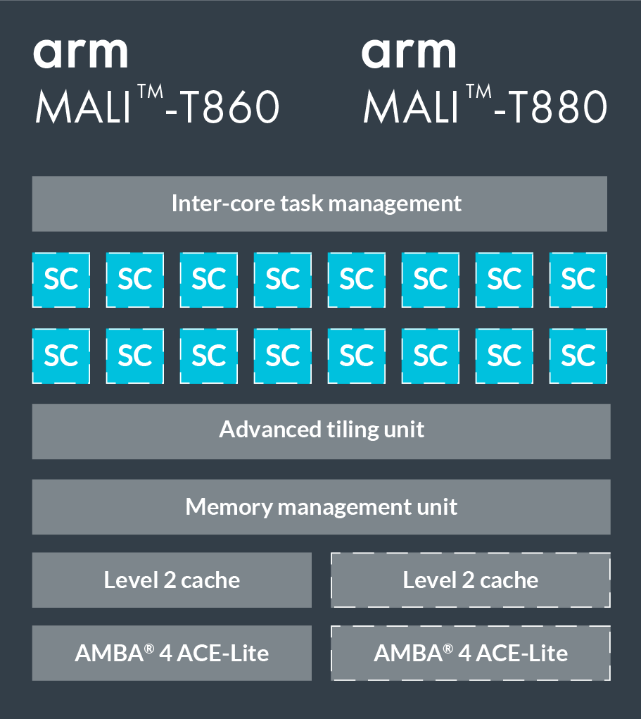
Architecture
Figure 1 is an overview of the Mali Architecture on T860 and T880. The GPUs are scalable up to 16 coherent shader cores. Inside each shader core, there are 2 or 3 arithmetic pipelines, 1 load/store pipeline and 1 texture pipeline (so-called TriPipe). The ALU in each arithmetic pipeline has four 128-bit vector units and one scalar units.
We use OpenCL for GPU computing. When mapping to OpenCL model, each shader core executes one or several work groups. Each shader core supports up to 384 concurrently executing threads. Each work item in OpenCL typically maps to a single thread on a Mali GPU. The Mali GPUs use a VLIW (Very Long Instruction Word) architecture. Each instruction word contains multiple operations. The Mali GPUs also use SIMD, so that most arithmetic instructions operate on multiple data elements simultaneously. [1]
Difference with NVIDIA’s GPUs
Here are some differences that we should concern when writing OpenCL code for Mali GPUs, compared with writing for NVIDIA’s GPUs.
- Mali GPUs use an unified global memory. In NVIDIA’s GPUs, we usually copy data to shared memory, because NVIDIA’s GPUs have physically separate global memory, shared memory and register. In Mali, this copy does not improve performance and can be removed. Besides, Mali GPUs usually share the global memory with CPU, so there is no need for copying between CPU and GPU.
- Mali Midgrad GPUs are based on SIMD (Single Instruction Multiple Data) and need explicit vectorization. In NVIDIA CUDA, parallelism is achieved by SIMT (Single Instruction Multiple Thread), which does not require explicit vectorization. But also notice that the newer Mali Bitfrost GPUs are based on quad-style vectorization and does not require explicit vectorization.
- All threads in Mali GPUs have individual program counters. It means
the
warp sizeis 1, so that branch divergence is not a major problem.
Optimization : Convolution as Example
The convolution layer is the core of most deep neural networks and takes most of the computation time. So we take the convolution layer as example to demonstrate how common optimization techniques like packing, tiling, unrolling and vectorization are applied in TVM.
Im2Col with GEMM
A well-known algorithm for convolution layer is im2col, which converts the little 3D input cubes to columns of a matrix and perform a GEMM. The advantage of this method is easy utilization of highly optimized BLAS library. However, the memory redundancy (9x memory for 3x3 kernel) is awful.
Spatial Packing
Instead, we adopt a method to calculate the convolution, and apply the optimization techniques step by step. A convolution layer in VGG-16 is used as tuning case, whose configuration is listed below. We assume the batch size is 1 for inference.
| Input Shape | Output Shape | Kernel Size | Stride | Padding |
|---|---|---|---|---|
| 56x56x256 | 56x56x256 | 3x3 | (1, 1) | (1, 1) |
As a baseline, we also list the performance of this layer in Arm Compute Library.
| Kernel | Cost (second) | GFLOPS |
|---|---|---|
| GEMM method in ARMComputeLib | 0.1821 | 20.3111 |
Declare the computation: tiling and packing
Tiling and packing are two methods intended for better memory access. Tiling separates the whole computation into small blocks for better datareuse. Packing re-layouts the input matrices according to the tiling so that we can access the memory sequentially, which reduces cache miss rate.
We do tiling on the width dimension of the input image and CO dimension
of the filter matrix. This is described by tvm.compute.
# set tiling factor
VH = 1
VW = VC = 4

# get input shape
 _, CI, IH, IW = data.shape
CO, CI, KH, KW = kernel.shape
TH = IH + 2 * H_PAD
TW = IW + 2 * W_PAD

# calc output shape
OH = (IH + 2*H_PAD - KH) // H_STR + 1
OW = (IW + 2*W_PAD - KW) // W_STR + 1

# data shape after packing
dvshape = (N, TH // (VH*H_STRIDE), TW // (VW*W_STRIDE), CI, VH*H_STRIDE+HCAT, VW*W_STRIDE+WCAT)

# kernel shape after packing
kvshape = (CO // VC, CI, KH, KW, VC)

ovshape = (N, CO // VC, OH // VH, OW // VW, VH, VW, VC)
oshape = (N, CO, OH, OW)

# define packing
data_vec = tvm.compute(dvshape, lambda n, h, w, ci, vh, vw:
    data_pad[n][ci][h*VH*H_STRIDE+vh][w*VW*W_STRIDE+vw], name='data_vec')

kernel_vec = tvm.compute(kvshape, lambda co, ci, kh, kw, vc:
    kernel[co*VC+vc][ci][kh][kw], name='kernel_vec')

# define convolution
ci = tvm.reduce_axis((0, CI), name='ci')
kh = tvm.reduce_axis((0, KH), name='kh')
kw = tvm.reduce_axis((0, KW), name='kw')

conv = tvm.compute(ovshape, lambda n, co, h, w, vh, vw, vc:
    tvm.sum(data_vec[n, h, w, ci, vh*H_STRIDE+kh, vw*W_STRIDE+kw].astype(out_dtype) *
            kernel_vec[co, ci, kh, kw, vc].astype(out_dtype),
            axis=[ci, kh, kw]), name='conv')

# unpack to correct layout
output = tvm.compute(oshape, lambda n, co, h, w:
                     conv[n][co//VC][h/VH][w//VW][h%VH][w%VW][co%VC],
                     name='output_unpack', tag='direct_conv_output')
We can inspect the defined IR by
print(tvm.lower(s, [data, kernel, output], simple_mode=True))
I pick the convolution part here.
produce conv {
  for (co, 0, 64) {
    for (h, 0, 56) {
      for (w, 0, 14) {
        for (vw.init, 0, 4) {
          for (vc.init, 0, 4) {
            conv[((((((((co*56) + h)*14) + w)*4) + vw.init)*4) + vc.init)] = 0.000000f
          }
        }
        for (ci, 0, 256) {
          for (kh, 0, 3) {
            for (kw, 0, 3) {
              for (vw, 0, 4) {
                for (vc, 0, 4) {
                  conv[((((((((co*56) + h)*14) + w)*4) + vw)*4) + vc)] = (conv[((((((((co*56) + h)*14) + w)*4) + vw)*4) + vc)] + (data_vec[(((((((((h*14) + w)*256) + ci)*3) + kh)*6) + kw) + vw)]*kernel_vec[((((((((co*256) + ci)*3) + kh)*3) + kw)*4) + vc)]))
                }
              }
            }
          }
        }
      }
    }
  }
}
Kernel 1: bind thread
In TVM, we declare the computation at first and then schedule it. This mechanism decouples the algorithm and implementation detail. (This idea is from Halide).
The following schedule simply binds axes to GPU threads, so that our code can run on Mali GPU.
# helper function for binding thread
def tile_and_bind3d(s, tensor, z, y, x, z_factor=2, y_factor=None, x_factor=None):
    """ tile and bind 3d """
    y_factor = y_factor or z_factor
    x_factor = x_factor or y_factor
    zo, zi = s[tensor].split(z, z_factor)
    yo, yi = s[tensor].split(y, y_factor)
    xo, xi = s[tensor].split(x, x_factor)
    s[tensor].bind(zo, tvm.thread_axis("blockIdx.z"))
    s[tensor].bind(zi, tvm.thread_axis("threadIdx.z"))
    s[tensor].bind(yo, tvm.thread_axis("blockIdx.y"))
    s[tensor].bind(yi, tvm.thread_axis("threadIdx.y"))
    s[tensor].bind(xo, tvm.thread_axis("blockIdx.x"))
    s[tensor].bind(xi, tvm.thread_axis("threadIdx.x"))

# set tunable parameter
num_thread = 8

# schedule data packing
_, h, w, ci, vh, vw = s[data_vec].op.axis
tile_and_bind3d(s, data_vec, h, w, ci, 1)

# schedule kernel packing
co, ci, kh, kw, vc = s[kernel_vec].op.axis
tile_and_bind(s, kernel_vec, co, ci, 1)

# schedule conv
_, c, h, w, vh, vw, vc = s[conv].op.axis
kc, kh, kw = s[conv].op.reduce_axis

s[conv].reorder(_, c, h, w, vh, kc, kh, kw, vw, vc)
tile_and_bind3d(s, conv, c, h, w, num_thread, 1, 1)

_, co, oh, ow = s[output].op.axis
tile_and_bind3d(s, output, co, oh, ow, num_thread, 1, 1)
With this schedule, our code can run now, but the performance is terrible.
| Kernel | Cost (second) | GFLOPS | speedup |
|---|---|---|---|
| GEMM method in ARMComputeLib | 0.1821 | 20.3111 | 1x |
| Kernel 1: simple bind | 5.6154 | 0.6588 | 0.03x |
Kernel 2: unrolling
Loop unrolling can reduce the instructions for loop control, reduce
branch penalties and hide latency in reading memory.
In TVM, this can be done easily by calling s.unroll(axis)
# set tunable parameter
num_thread = 8

# schedule data packing
_, h, w, ci, vh, vw = s[data_vec].op.axis
tile_and_bind3d(s, data_vec, h, w, ci, 1)

"""!! ADD UNROLL HERE !!"""
s[data_vec].unroll(vw)

# schedule kernel packing
co, ci, kh, kw, vc = s[kernel_vec].op.axis
tile_and_bind(s, kernel_vec, co, ci, 1)

"""!! ADD UNROLL HERE !!"""
s[kernel_vec].unroll(kh)
s[kernel_vec].unroll(kw)
s[kernel_vec].unroll(vc)

# schedule conv
_, c, h, w, vh, vw, vc = s[conv].op.axis
kc, kh, kw = s[conv].op.reduce_axis

s[conv].reorder(_, c, h, w, vh, kc, kh, kw, vw, vc)
tile_and_bind3d(s, conv, c, h, w, num_thread, 1, 1)

"""!! ADD UNROLL HERE !!"""
s[conv].unroll(kh)
s[conv].unroll(kw)
s[conv].unroll(vw)
s[conv].unroll(vc)

_, co, oh, ow = s[output].op.axis
tile_and_bind3d(s, output, co, oh, ow, num_thread, 1, 1)
| Kernel | Cost (second) | GFLOPS | speedup |
|---|---|---|---|
| GEMM method in ARMComputeLib | 0.1821 | 20.3111 | 1x |
| Kernel 1: simple bind | 5.6154 | 0.6588 | 0.03x |
| Kernel 2: + unrolling | 0.3707 | 9.9796 | 0.49x |
Kernel3: vectorization
As mentioned before, we need to do vectorization explictly in order to achieve the best performance on Mali GPU.
# set tunable parameter
num_thread = 8

# schedule data packing
_, h, w, ci, vh, vw = s[data_vec].op.axis
tile_and_bind3d(s, data_vec, h, w, ci, 1)

# unroll
s[data_vec].unroll(vw)

# schedule kernel packing
co, ci, kh, kw, vc = s[kernel_vec].op.axis
tile_and_bind(s, kernel_vec, co, ci, 1)

# unroll
s[kernel_vec].unroll(kh)
s[kernel_vec].unroll(kw)
"""!! VECTORIZE HERE !!"""
s[kernel_vec].vectorize(vc)

# schedule conv
_, c, h, w, vh, vw, vc = s[conv].op.axis
kc, kh, kw = s[conv].op.reduce_axis

s[conv].reorder(_, c, h, w, vh, kc, kh, kw, vw, vc)
tile_and_bind3d(s, conv, c, h, w, num_thread, 1, 1)

# unroll
s[conv].unroll(kh)
s[conv].unroll(kw)
s[conv].unroll(vw)
"""!! VECTORIZE HERE !!"""
s[conv].vectorize(vc)

_, co, oh, ow = s[output].op.axis
tile_and_bind3d(s, output, co, oh, ow, num_thread, 1, 1)
| Kernel | Cost (second) | GFLOPS | speedup |
|---|---|---|---|
| GEMM method in ARMComputeLib | 0.1821 | 20.3111 | 1x |
| Kernel 1: simple bind | 5.6154 | 0.6588 | 0.03x |
| Kernel 2: + unrolling | 0.3707 | 9.9796 | 0.49x |
| Kernel 3: + vectorization | 0.1304 | 28.3679 | 1.40x |
How to set the tunable parameter
As for the tunable parameters above, some can be calculated.
For the vectorized dimension VC, we should fill the 128-bit register,
so it can be set as 128/32=4 for float32 and 128/16=8 for float16.
But more often we cannot determine the optimal value, due to the complicated runtime. We use grid search in TVM. It can be done extremely effective since we write python code in TVM’s high-level IR rather than direct OpenCL code.
The generated OpenCL code
We can view the generated OpenCL code by
print(func.imported_modules[0].get_source())
The OpenCL code is too long to be pasted here, and it is hard to read due to heavy unrolling. If interested, you can view it here.
End-to-End Benchmarking
In this section, we compare the comprehensive performance between different backends on some popular deep neural networks. Our test environment is
Firefly-RK3399 4G
CPU: dual-core Cortex-A72 + quad-core Cortex-A53
GPU: Mali-T860MP4

Arm Compute Library : v17.12
MXNet: v1.0.1
Openblas: v0.2.18
We use NNVM and TVM to do end-to-end compilation.
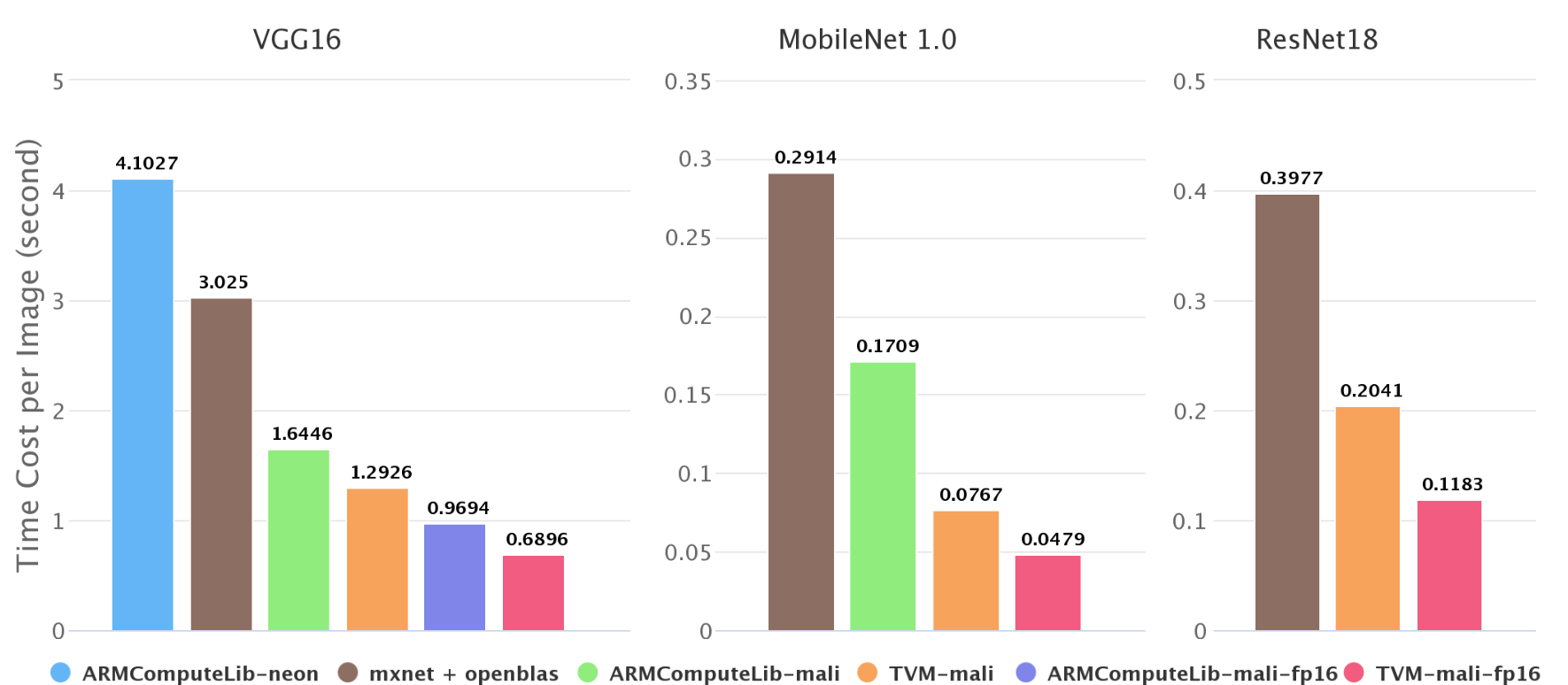
Performance
As shown in Figure 2, we test the inference speed on ImageNet. On Firefly-RK3399, Mali GPU can be 2x ~ 4x faster than 6-core big.LITTLE CPU. Our end-to-end pipeline is 1.4x ~ 2.2x faster than Arm Compute Library. We try both GEMM and direct method of convolution layer in Arm Compute Library, GEMM method is always faster than direct method in these test cases, so we only plot the result of GEMM method.
Some results, like resnet18 on Arm Compute Library, are missing in the Figure 2. It is because the graph runtime of Arm Compute Library does not support skip connection currently and has a poor neon implementation of depthwise convolution. This also reflects the advantage of NNVM software stack.
Half-Precision Performance
Precision in deep neural networks is not very important, especially for the inference on mobile devices. Using low-precision arithmetic can make the inference much faster. We also test the half-precision floating number on Mali GPU.
| model | backend | Time Cost per Image (second) | speed up to FP32 |
|---|---|---|---|
| vgg16 | ACM-mali | 0.9694 | 1.69 |
| vgg16 | TVM-mali | 0.6896 | 1.87x |
| MobileNet 1.0 | TVM-mali | 0.0479 | 1.60x |
| ResNet18 | TVM-mali | 0.1183 | 1.73x |
In theory, FP16 can both double peak compute and halve memory consumption, so that doubling the speed. But it needs good input shape for longer vectorization and fine-tuning some parameters.
Further Work on Mobile Devices
We should admit that there is still some room for improvement, mainly at the graph level, such as model compression and weight prelayout. Further improvement in NNVM will try to solve these problems.
Show me the code
Bio & Acknowledgement
Lianmin Zheng is an undergraduate student at SJTU Apex lab. He is interested in machine learning and building computer system.
The author has many thanks to Tianqi Chen for his helpful advice and Yizhi Liu for his earlier work.